In almost every industry in the world, more often than not, you will be faced with comparing data. Whatever your department is, company data will need to be adjusted based on current needs.
In this post, we are going to show you how two tables are connected one another, just like in the real world. Let’s say you have these employee data and the assessment report of some employees who have finished doing the assessment. These two data are not usually together, one could be in the database, while the other could be sent by your superior who want to know more about the data. But this time to make it easy for learning purpose, we show it together in one sheet.

We can see that the table Assessment Report on the right doesn’t include employee names. This is very common in almost every company, since data like Assessment Report usually follows database many to one principal to save space and practicality in the database.
Now let’s say your manager sent you the Assessment Report in excel file, and you have your own employee data containing employee id, first name, and last name. Your manager wants to know who has conducted the assessment along with the test result, because he obviously cannot tell who they are only from the employee id.
You can filter the employee id individually and copy paste the last and first names, but when there are hundreds or thousands of data in the Assessment Report, you need to utilize an excel formula. There are two possible formulas to compare these two data. One of them is VLOOKUP that I already covered in my previous post here : Excel : Using VlookUp Formula to Perform Data Comparison. The other one is the one that I am going to show you now, which is the INDEX and MATCH formula.
So basically this is what you need to type in the new last name field in Assessment Report data.
=INDEX(table_array,MATCH(lookup_value,column_array,[match_type]),column_num)Or in our case, this is the exact formula we need to type.
=INDEX($A$4:$C$16,MATCH(E4,$A$4:$A$16,0),2)We can see that we filled the [match_type] parameter with 0. This is to indicate the formula to find the exact match instead of the closest match or approximate value. I you are new to this and want to only find the exact value like employee ID, make sure to always use FALSE or 0.

After verifying that the first row of last name is indeed correct as it is in the employee data, you can copy and paste the cell to the other rows below it. Next, you can proceed with the first name.
The First Name field is similar to last name, except the column_num needs to be set as 3, since the field First Name is in the third column that was selected in the dataset or table_array.
=INDEX($A$4:$C$16,MATCH($E4,$A$4:$A$16,0),3)
Notice that the only difference between last name and first name is the col_index_num, since it indicates the column number of table_array, or in this case, it is the Employee Data table.
When you are done with your formula, hit enter and copy that first row of First Name and paste it into all rows below it.

Before we end this post, there is one more thing to show you. In this kind of situation, sometimes we need to know which employee has done certain test. For example, we are asked if an employee named Bret Favre has done any of his assessments or not. This example can also easily be search with INDEX and MATCH formula. Just add a column next to First Name in the Employee data table, then type the following formula for our specific case.
=INDEX($F$4:$J$16,MATCH(A4,F4:F16,0),2)This is the result you get with the above formula.
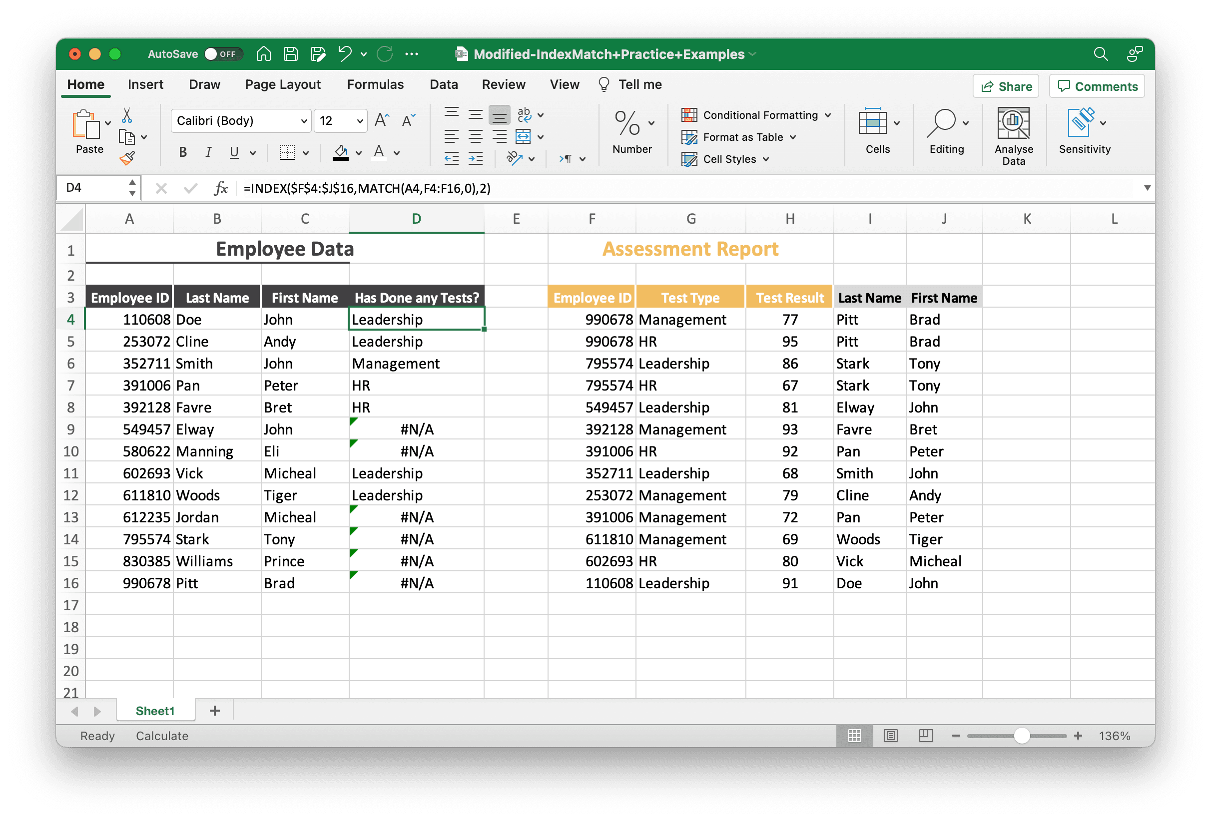
Notice that if an employee is not available anywhere in the Assessment Report table, the result will be N/A. This is very easy to make a quick scan of who has not done any of their tests at all.
In summary, I can guarantee you that if you work in a company or have your own business, you will most likely face this kind of situation where you need to extract data from other table. This INDEX and MATCH formula is indeed very simple yet very popular, and you definitely can make use of it very often. This formula also has an advantage compared to the VLOOKUP formula : the lookup value doesn’t need to be on the most left hand side or first column of the table. It could be anywhere. Although this is a slightly more advanced formula than VLOOKUP, a lot of people uses it for daily data comparation, because it is still very simple and doesn’t need a lot of characters to type.