Conditional Formatting by Value : Automated Cell Formatting in Excel

In the world of spreadsheets, Excel stands out as a powerhouse of functionality and versatility. One of its most powerful features, Conditional Formatting, allows users to dynamically highlight and format cells based on specific conditions or criteria. With this tool at your disposal, you can effectively visualize and analyze data, making important insights leap off the screen. In this article, we will dive into the world of Excel Conditional Formatting, exploring its various applications and sharing tips to help you make the most of this invaluable feature.

Understanding Conditional Formatting

Conditional Formatting enables you to format cells based on their values, formulas, or specific rules. By setting up conditions, Excel automatically applies formatting, creating visual cues that make patterns, trends, and anomalies in your data readily apparent. Whether you’re dealing with numerical data, dates, or text, Conditional Formatting empowers you to highlight important information effortlessly.

Applying Basic Conditional Formatting:

To apply basic Conditional Formatting, follow these steps:

1. Select the range of cells you want to format.
2. From the Excel Ribbon, go to the “Home” tab, and click on the “Conditional Formatting” dropdown menu.
3. Choose the desired formatting option, such as “Highlight Cells Rules” or “Data Bars.”
4. Select the specific condition or criteria, and set the formatting style and color scheme.
5. Click “OK” to apply the Conditional Formatting to the selected cells.

Example

Highlighting Values above a Certain Threshold:

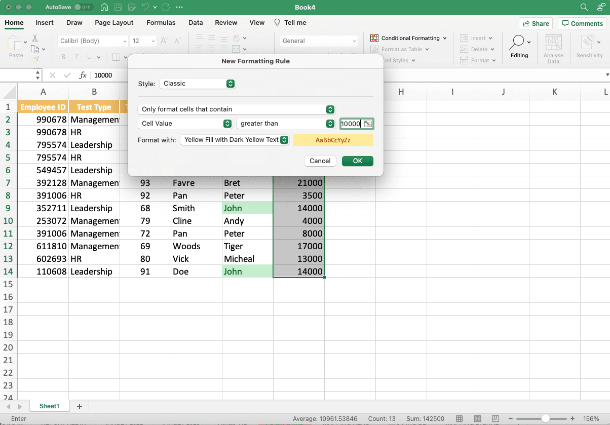
Suppose you have a column of sales data, and you want to highlight all values above $10,000 in green. Using Conditional Formatting:

1. Select the sales column.
2. Go to the “Home” tab, click on “Conditional Formatting,” and choose “Highlight Cells Rules” > “Greater Than.”
3. In the dialog box, enter “10000” as the value.
4. Select the desired formatting style, such as “Yellow Fill with Dark Yellow Text.”
5. Click “OK” to apply the formatting. All values above $10,000 will now be highlighted in yellow.

Customizing Conditional Formatting Rules

Excel allows you to create custom Conditional Formatting rules based on specific criteria. To create a custom rule:

1. Select the range of cells.
2. Go to the “Home” tab, click on “Conditional Formatting,” and choose “New Rule.”
3. Select the rule type, such as “Format only cells that contain” or “Use a formula to determine which cells to format.”
4. Enter the desired condition or formula in the respective field.
5. Specify the formatting options, such as font color, background color, or data bars.
6. Click “OK” to apply the custom Conditional Formatting rule.

Example

Highlighting Duplicate Entries

Suppose you have a list of customer names, and you want to highlight duplicate entries. Using Conditional Formatting:

1. Select the customer names column.
2. Go to the “Home” tab, click on “Conditional Formatting,” and choose “Highlight Cells Rules” > “Duplicate Values.”
3. Select the desired formatting style, such as “Light Red Fill.”
4. Click “OK” to apply the formatting. All duplicate customer names will now be highlighted.

Tips and Tricks

1. Manage complex formatting rules by prioritizing them using the “Manage Rules” option.
2. Copy and paste Conditional Formatting across cells and sheets using the “Format Painter” tool.
3. Use color scales or icon sets to represent data ranges and create visually appealing heatmaps.
4. Experiment with different formatting options and styles to find the best way to represent your data effectively.

Conclusion

Excel’s Conditional Formatting feature opens a world of possibilities for visual data analysis. By effectively highlighting and formatting cells based on specific conditions, you can unlock valuable insights and present your data with clarity and impact. Whether you’re a business analyst, researcher, or spreadsheet enthusiast, mastering Conditional Formatting will undoubtedly take your Excel skills to new heights. Embrace this powerful tool, follow the instructions, and explore the examples to transform your data analysis journey.

Explore our Excel post category to excel in this application for your professional pursuits.