
Even if You are new to Microsoft Excel, You have probably heard of Pivot Table. This feature is a powerful tool to make a report to summarize Your data.

Sample DataFor example, You have this data above. To summarize the data for Your boss, or just to make it easier to You to read, select anywhere in the data, click on Insert -> Pivot Table.

You can modify Pivot Table options to according to your wishes, but to make it simple, You can just click Ok.

This pivot table block will appear, along with Pivot Table fields on the far right.
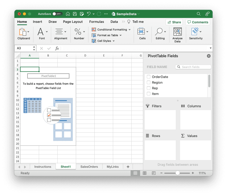
There are five blocks available at the far right panel, as we can see in Pivot Table Fields. The way it works is we need to drag any fields from the Available Field Name on the top row of the panel, according to where it belongs.
- Available Field Name (top row)
- Filters
- Columns
- Rows
- Values
The thing You need to remember is Rows and Columns block must be filled by one or more fields. For example, if You want to see how many units are available in every region, You just need to drag the Region field into Rows block, and the Units field into Columns block.

As You can see, Pivot table shown above is the minimum and simplest pivot table You can make in a few seconds. You can adjust the filters, columns, rows, and values according to your needs.
There are lots of advanced usages of Pivot Table, which I will show You in other future posts. This feature is essential for all companies, including big enterprises, since Excel is still relevant in today’s reporting. If you want to check out other tips about Microsoft Excel, check out our category about Microsoft Excel here.


Thank you for the simplest yet detailed explanation about pivot table!